🎯 Estimate Corrected MMs or AMCEs
In conjoint analysis, default MMs and AMCEs can be biased due to measurement error from intra-respondent variability.
projoint corrects for this bias automatically.
The following instructions apply to choice-level data. What if you have profile-level data?ⓘ Our FAQ Page has instructions to estimate and visualize profile-level QOIs.
📦 Prepare Example Data
Outcome naming & order (important)
- List
.outcomesin the order questions were asked.
- If you have a repeated task, its outcome must be the last element.
- For base tasks (all but last), the function reads the digits in each name as the task id (e.g.,
"choice4","Q4","task04"→ task 4).
- The repeated base task is inferred from the first base outcome’s digits. The repeated outcome itself need not contain digits—only its position (last) matters.
- Outcome strings should end with your choice labels; by default we parse the last character and expect
"A"/"B". If your survey uses"1"/"2"(or other endings), set.choice_labelsaccordingly.
Examples
# Standard order; repeated = task 1
data("exampleData1")
outcomes <- c(paste0("choice", 1:8), "choice1_repeated_flipped")
out1 <- reshape_projoint(exampleData1, outcomes)
🛠️ Why Use IDs (e.g., att1, level1)?
Before estimating quantities, it’s important to understand how attribute and level IDs work inside projoint.
We recommend working with attribute IDs rather than actual text labels because:
- Safer against special characters, languages, or typos
- Allows multiple attributes to have identical labels (e.g., “High” for both “Teaching Quality” and “Research Quality”)
Check attribute-level mappings:
out1$labels## # A tibble: 24 × 4
## attribute level attribute_id level_id
## <chr> <chr> <chr> <chr>
## 1 Housing Cost 15% of pre-tax income att1 att1:leve…
## 2 Housing Cost 30% of pre-tax income att1 att1:leve…
## 3 Housing Cost 40% of pre-tax income att1 att1:leve…
## 4 Presidential Vote (2020) 30% Democrat, 70% Republican att2 att2:leve…
## 5 Presidential Vote (2020) 50% Democrat, 50% Republican att2 att2:leve…
## 6 Presidential Vote (2020) 70% Democrat, 30% Republican att2 att2:leve…
## 7 Racial Composition 50% White, 50% Nonwhite att3 att3:leve…
## 8 Racial Composition 75% White, 25% Nonwhite att3 att3:leve…
## 9 Racial Composition 90% White, 10% Nonwhite att3 att3:leve…
## 10 Racial Composition 96% White, 4% Nonwhite att3 att3:leve…
## # ℹ 14 more rowsYou can also save these labels for easier editing:
save_labels(out1, "labels.csv")📈 Estimate Marginal Means (MMs)
Choice-Level MMs (Specific Level)
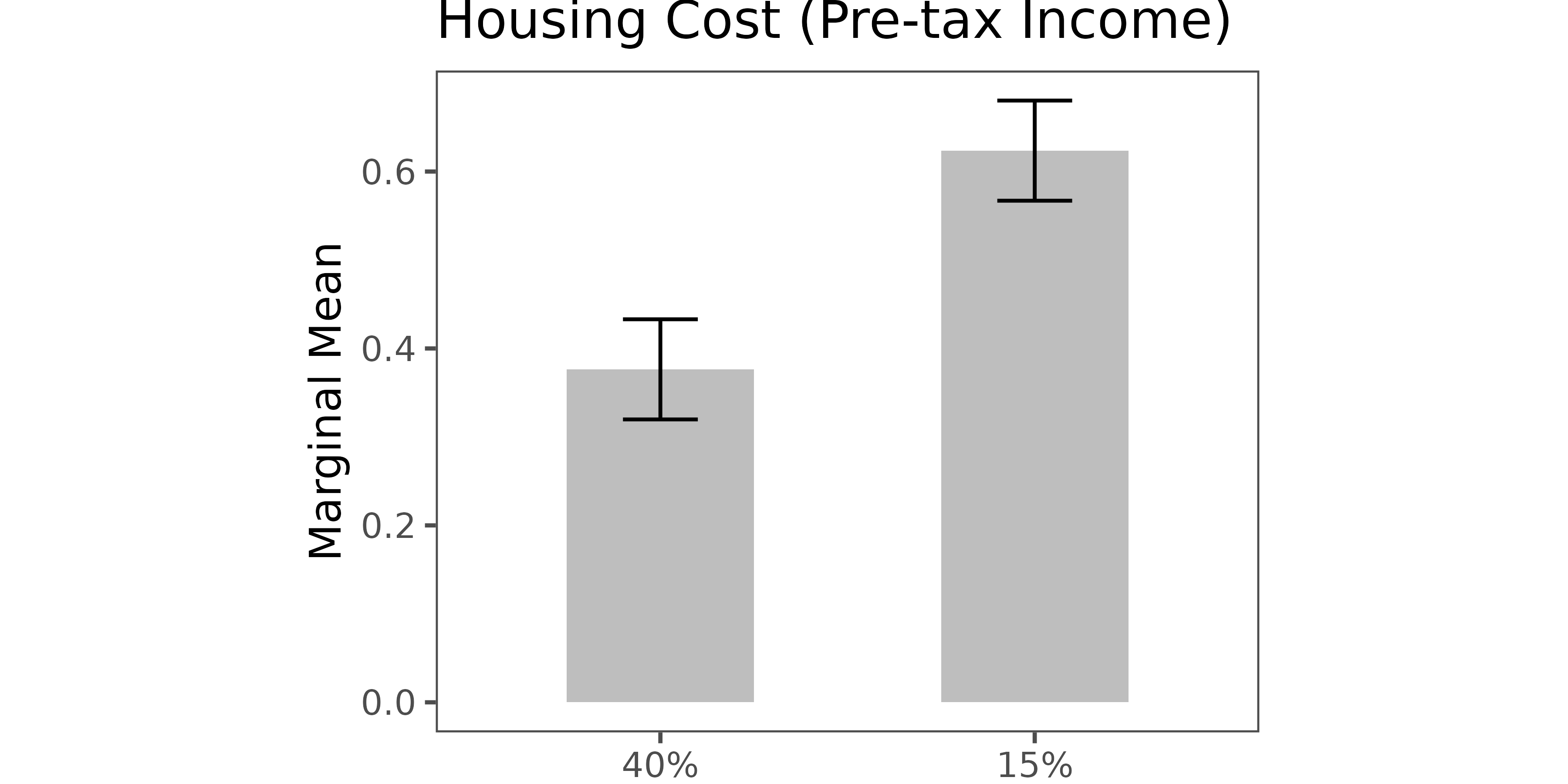
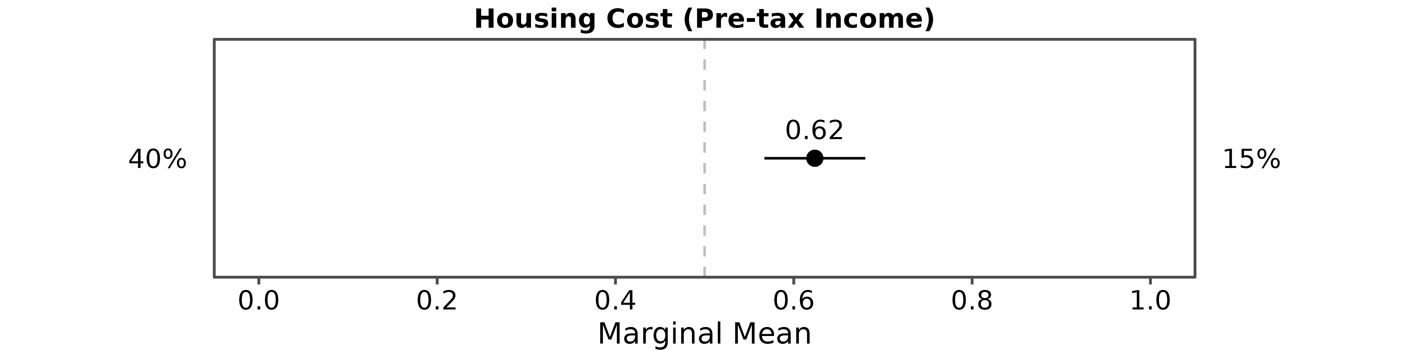
Suppose you want to estimate, within a given profile pair, the
probability of choosing a profile that includes “40% of pre-tax income”
(level3) for Housing Cost (att1) rather than
one that includes “15% of pre-tax income” (level1) for the
same attribute, averaging over all combinations of the other attributes
and across respondents; then use the following code:
qoi <- set_qoi(
  .structure = "choice_level",
  .att_choose = "att1",
  .lev_choose = "level3",
  .att_notchoose = "att1",
  .lev_notchoose = "level1"
)

mm2 <- projoint(out1, qoi)
print(mm2)
##
## Projoint results object
## -------------------------
## Estimand: mm
## Structure: choice_level
## Standard error method: analytical
## IRR: Estimated
## Tau: 0.172
## Number of estimates: 2
summary(mm2)##
## Summary of Projoint Estimates
## ------------------------------
## Estimand: mm
## Structure: choice_level
## Standard error method: analytical
## SE type (lm_robust): CR2 (clustered by id)
## IRR: Estimated
## Tau: 0.172## # A tibble: 2 × 7
## estimand estimate se conf.low conf.high att_level_choose
## <chr> <dbl> <dbl> <dbl> <dbl> <chr>
## 1 mm_uncorrected 0.419 0.0197 0.380 0.458 att1:level3
## 2 mm_corrected 0.376 0.0308 0.316 0.437 att1:level3
## # ℹ 1 more variable: att_level_notchoose <chr>📉 Estimate AMCEs
Choice-Level AMCEs (Specific Level)
Suppose you want to quantify how the choice probability changes between the following profile pairs:
- choosing a profile that includes “40% of pre-tax income”
(
level3) for Housing Cost (att1) versus one that includes “15% of pre-tax income” (level1) for Housing Cost (att1); and - [baseline] choosing a profile that includes “30% of pre-tax income”
(
level2) for Housing Cost (att1) versus one that includes “15% of pre-tax income” (level1) for Housing Cost (att1);
averaging over all combinations of the other attributes and across respondents. Then write the following code:
qoi <- set_qoi(
  .structure = "choice_level",
  .estimand = "amce",
  .att_choose = "att1",
  .lev_choose = "level3",
  .att_notchoose = "att1",
  .lev_notchoose = "level1",
  .att_choose_b = "att1",
  .lev_choose_b = "level2",
  .att_notchoose_b = "att1",
  .lev_notchoose_b = "level1"
)

amce2 <- projoint(out1, qoi)
print(amce2)
##
## Projoint results object
## -------------------------
## Estimand: amce
## Structure: choice_level
## Standard error method: analytical
## IRR: Estimated
## Tau: 0.172
## Number of estimates: 2
summary(amce2)##
## Summary of Projoint Estimates
## ------------------------------
## Estimand: amce
## Structure: choice_level
## Standard error method: analytical
## SE type (lm_robust): CR2 (clustered by id)
## IRR: Estimated
## Tau: 0.172## # A tibble: 2 × 9
## estimand estimate se conf.low conf.high att_level_choose
## <chr> <dbl> <dbl> <dbl> <dbl> <chr>
## 1 amce_uncorrected -0.0135 0.0269 -0.0665 0.0394 att1:level3
## 2 amce_corrected -0.0206 0.0412 -0.102 0.0604 att1:level3
## # ℹ 3 more variables: att_level_notchoose <chr>,
## # att_level_choose_baseline <chr>, att_level_notchoose_baseline <chr>🔎 Predict Intra-Respondent Reliability (IRR)
If your design does not include a repeated task, you can predict IRR using predict_tau(), based on observed respondent behavior.
Predict IRR Using predict_tau()
data(out1_arranged)
predicted_irr <- predict_tau(out1_arranged)

print(predicted_irr)
## Tau estimated using the extrapolation method: 0.743
summary(predicted_irr)## # A tibble: 8 × 2
## x predicted
## <int> <dbl>
## 1 0 0.743
## 2 1 0.709
## 3 2 0.675
## 4 3 0.640
## 5 4 0.606
## 6 5 0.572
## 7 6 0.537
## 8 7 0.503
plot(predicted_irr)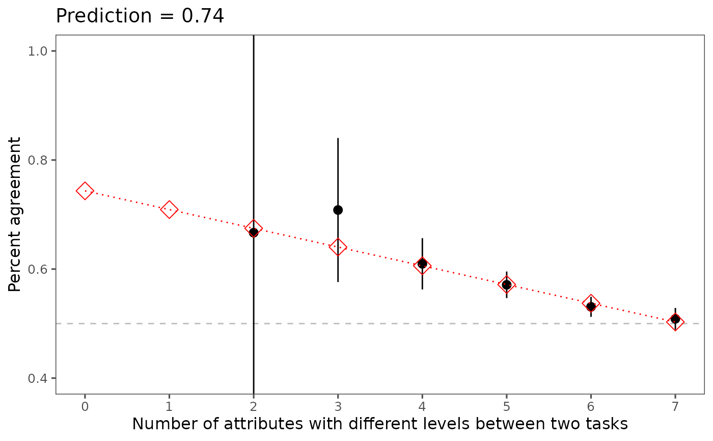
🎨 Visualize MMs or AMCEs
The projoint package provides ready-to-publish plotting tools for conjoint analysis results.
Note: The current version
of projoint supports plotting choice-level MMs
only.
Support for choice-level AMCEs will be available in
future updates!
⚖️ Choice-Level Analysis
Estimate
- Specify your quantity of interest:
qoi_mm <- set_qoi(
  .structure = "choice_level", # default
  .att_choose = "att1",
  .lev_choose = "level1",
  .att_notchoose = "att1",
  .lev_notchoose = "level3"
)- Estimate
choice_mm <- projoint(
  .data = out1_arranged,
  .qoi = qoi_mm,
  .ignore_position = TRUE
)
🏠 Home: Home