What’s the difference between “profile-level” and “choice-level” conjoint analysis??
Choice-level analysis is simpler, easier, and more powerful than profile-level analysis.
Conjoint designs originated in market research and psychology where each respondent is asked to rate each of two different profiles (e.g., two products). Each of the two ratings provided separate information, and the two are analyzed as separate observations. Researchers with this profile-level design find it convenient to arrange their data with one profile per row, and thus twice as many rows as respondents.
Unfortunately, when social scientists adopted the conjoint survey design, they kept the same profile-level design but changed the outcome measure from separate ratings to a single choice between the two profiles (e.g., to reflect a voter choice between two candidates). In this situation, respondents asked to make one choice between the two profiles that are exactly dependent, as choosing one necessarily meant not choosing the other (e.g., in a two-candidate partisan election, one observation would be “Democrat” and the other would be “not the Republican”). Using this profile-level design with 2*n rows but only n independent observations requires the introduction of complicated statistical procedures to correct for the dependence induced solely by the researcher’s decision to organize the data in this complicated way.
We recommend the much simpler and more powerful choice-level design. The idea is to arrange data at the level of the respondent’s choice, so that each row in the data matrix includes information about one choice (and both profiles together, with n observations and n rows). Our AJPS article clarifies this point, shows how this choice-level analysis vastly simplifies the notation, statistical analysis procedures, and intuition, and greatly expands the substantive questions conjoint analysis be used to answer.
What if I have profile-level data?
Transform your data to choice-level, which is simpler and more powerful. To replicate old analyses, you can also use our profile-level tools
Profile-Level MMs (All Levels)
##
## Projoint results object
## -------------------------
## Estimand:  mm
## Structure:  profile_level
## Standard error method:  analytical
## IRR:  Estimated
## Tau:  0.172
## Number of estimates:  48
summary(mm0)##
## Summary of Projoint Estimates
## ------------------------------
## Estimand: mm
## Structure: profile_level
## Standard error method: analytical
## SE type (lm_robust): CR2 (clustered by id)
## IRR: Estimated
## Tau: 0.172## # A tibble: 48 × 6
## estimand estimate se conf.low conf.high att_level_choose
## <chr> <dbl> <dbl> <dbl> <dbl> <chr>
## 1 mm_uncorrected 0.574 0.0142 0.546 0.602 att1:level1
## 2 mm_corrected 0.614 0.0219 0.571 0.657 att1:level1
## 3 mm_uncorrected 0.485 0.0136 0.458 0.511 att1:level2
## 4 mm_corrected 0.477 0.0207 0.436 0.517 att1:level2
## 5 mm_uncorrected 0.445 0.0142 0.417 0.472 att1:level3
## 6 mm_corrected 0.416 0.0219 0.372 0.459 att1:level3
## 7 mm_uncorrected 0.489 0.0150 0.459 0.518 att2:level1
## 8 mm_corrected 0.483 0.0229 0.438 0.528 att2:level1
## 9 mm_uncorrected 0.524 0.0133 0.497 0.550 att2:level2
## 10 mm_corrected 0.536 0.0203 0.496 0.576 att2:level2
## # ℹ 38 more rowsProfile-Level MMs (Specific Level)
qoi_1 <- set_qoi(
  .structure = "profile_level",
  .estimand = "mm",
  .att_choose = "att1",
  .lev_choose = "level1"
)

mm1 <- projoint(out1, .qoi = qoi_1)
print(mm1)
##
## Projoint results object
## -------------------------
## Estimand: mm
## Structure: profile_level
## Standard error method: analytical
## IRR: Estimated
## Tau: 0.172
## Number of estimates: 2
summary(mm1)##
## Summary of Projoint Estimates
## ------------------------------
## Estimand: mm
## Structure: profile_level
## Standard error method: analytical
## SE type (lm_robust): CR2 (clustered by id)
## IRR: Estimated
## Tau: 0.172## # A tibble: 2 × 7
## estimand estimate se conf.low conf.high att_level_choose
## <chr> <dbl> <dbl> <dbl> <dbl> <chr>
## 1 mm_uncorrected 0.574 0.0142 0.546 0.602 att1:level1
## 2 mm_corrected 0.614 0.0219 0.571 0.657 att1:level1
## # ℹ 1 more variable: att_level_notchoose <chr>Profile-Level MMs (Specific Level, Manual IRR)
##
## Projoint results object
## -------------------------
## Estimand:  mm
## Structure:  profile_level
## Standard error method:  analytical
## IRR:  Assumed (0.75)
## Tau:  0.146
## Number of estimates:  2
summary(mm1b)##
## Summary of Projoint Estimates
## ------------------------------
## Estimand: mm
## Structure: profile_level
## Standard error method: analytical
## SE type (lm_robust): CR2 (clustered by id)
## IRR: Assumed (0.75)
## Tau: 0.146## # A tibble: 2 × 7
## estimand estimate se conf.low conf.high att_level_choose
## <chr> <dbl> <dbl> <dbl> <dbl> <chr>
## 1 mm_uncorrected 0.574 0.0142 0.546 0.602 att1:level1
## 2 mm_corrected 0.605 0.0201 0.566 0.645 att1:level1
## # ℹ 1 more variable: att_level_notchoose <chr>Profile-Level AMCEs (All Levels)
amce0 <- projoint(out1, .structure = "profile_level", .estimand = "amce")## Warning in pj_estimate(.data = .data, .structure = structure, .estimand =
## estimand, : AMCE analytical SEs: CR2 produced non-PSD/NA variances; fell back
## to se_type='stata' (then HC1 if needed).
print(amce0)##
## Projoint results object
## -------------------------
## Estimand: amce
## Structure: profile_level
## Standard error method: analytical
## IRR: Estimated
## Tau: 0.172
## Number of estimates: 34
summary(amce0)##
## Summary of Projoint Estimates
## ------------------------------
## Estimand: amce
## Structure: profile_level
## Standard error method: analytical
## SE type (lm_robust): CR2 (clustered by id)
## IRR: Estimated
## Tau: 0.172## # A tibble: 34 × 7
## estimand estimate se conf.low conf.high att_level_choose
## <chr> <dbl> <dbl> <dbl> <dbl> <chr>
## 1 amce_uncorrected -0.0899 0.0236 -0.136 -0.0435 att1:level2
## 2 amce_corrected -0.137 0.0360 -0.208 -0.0662 att1:level2
## 3 amce_uncorrected -0.130 0.0250 -0.179 -0.0808 att1:level3
## 4 amce_corrected -0.198 0.0386 -0.274 -0.122 att1:level3
## 5 amce_uncorrected 0.0348 0.0244 -0.0132 0.0828 att2:level2
## 6 amce_corrected 0.0530 0.0372 -0.0202 0.126 att2:level2
## 7 amce_uncorrected -0.00177 0.0263 -0.0536 0.0500 att2:level3
## 8 amce_corrected -0.00270 0.0402 -0.0817 0.0763 att2:level3
## 9 amce_uncorrected 0.0240 0.0233 -0.0218 0.0699 att3:level2
## 10 amce_corrected 0.0366 0.0357 -0.0336 0.107 att3:level2
## # ℹ 24 more rows
## # ℹ 1 more variable: att_level_choose_baseline <chr>Profile-Level AMCEs (Specific Level)
qoi_3 <- set_qoi(
  .structure = "profile_level",
  .estimand = "amce",
  .att_choose = "att1",
  .lev_choose = "level3",
  .att_choose_b = "att1",
  .lev_choose_b = "level1"
)

amce1 <- projoint(out1, .qoi = qoi_3)
print(amce1)
##
## Projoint results object
## -------------------------
## Estimand: amce
## Structure: profile_level
## Standard error method: analytical
## IRR: Estimated
## Tau: 0.172
## Number of estimates: 2
summary(amce1)##
## Summary of Projoint Estimates
## ------------------------------
## Estimand: amce
## Structure: profile_level
## Standard error method: analytical
## SE type (lm_robust): CR2 (clustered by id)
## IRR: Estimated
## Tau: 0.172## # A tibble: 2 × 9
## estimand estimate se conf.low conf.high att_level_choose
## <chr> <dbl> <dbl> <dbl> <dbl> <chr>
## 1 amce_uncorrected -0.130 0.0250 -0.179 -0.0808 att1:level3
## 2 amce_corrected -0.198 0.0386 -0.274 -0.122 att1:level3
## # ℹ 3 more variables: att_level_notchoose <chr>,
## # att_level_choose_baseline <chr>, att_level_notchoose_baseline <chr>Profile-Level AMCEs (Specific Level, Manual IRR)
##
## Projoint results object
## -------------------------
## Estimand:  amce
## Structure:  profile_level
## Standard error method:  analytical
## IRR:  Assumed (0.75)
## Tau:  0.146
## Number of estimates:  2
summary(amce1b)##
## Summary of Projoint Estimates
## ------------------------------
## Estimand: amce
## Structure: profile_level
## Standard error method: analytical
## SE type (lm_robust): CR2 (clustered by id)
## IRR: Assumed (0.75)
## Tau: 0.146## # A tibble: 2 × 9
## estimand estimate se conf.low conf.high att_level_choose
## <chr> <dbl> <dbl> <dbl> <dbl> <chr>
## 1 amce_uncorrected -0.130 0.0250 -0.179 -0.0808 att1:level3
## 2 amce_corrected -0.184 0.0353 -0.253 -0.114 att1:level3
## # ℹ 3 more variables: att_level_notchoose <chr>,
## # att_level_choose_baseline <chr>, att_level_notchoose_baseline <chr>
💡 Tip: When to Use
.by_var
Use .by_var only when comparing
profile-level MMs between two groups (e.g., Democrats
vs. Republicans).
.by_var is not
currently supported.
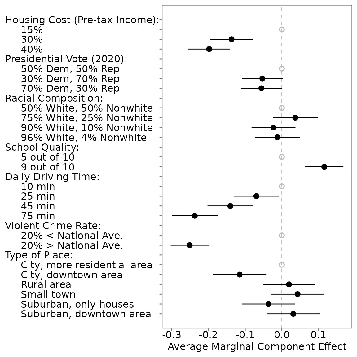
📈 Profile-Level MMs and AMCEs
Estimate
data("out1_arranged")
mm   <- projoint(out1_arranged, .structure = "profile_level")
amce <- projoint(out1_arranged, .structure = "profile_level", .estimand = "amce")
## Warning in pj_estimate(.data = .data, .structure = structure, .estimand =
## estimand, : AMCE analytical SEs: CR2 produced non-PSD/NA variances; fell back
## to se_type='stata' (then HC1 if needed).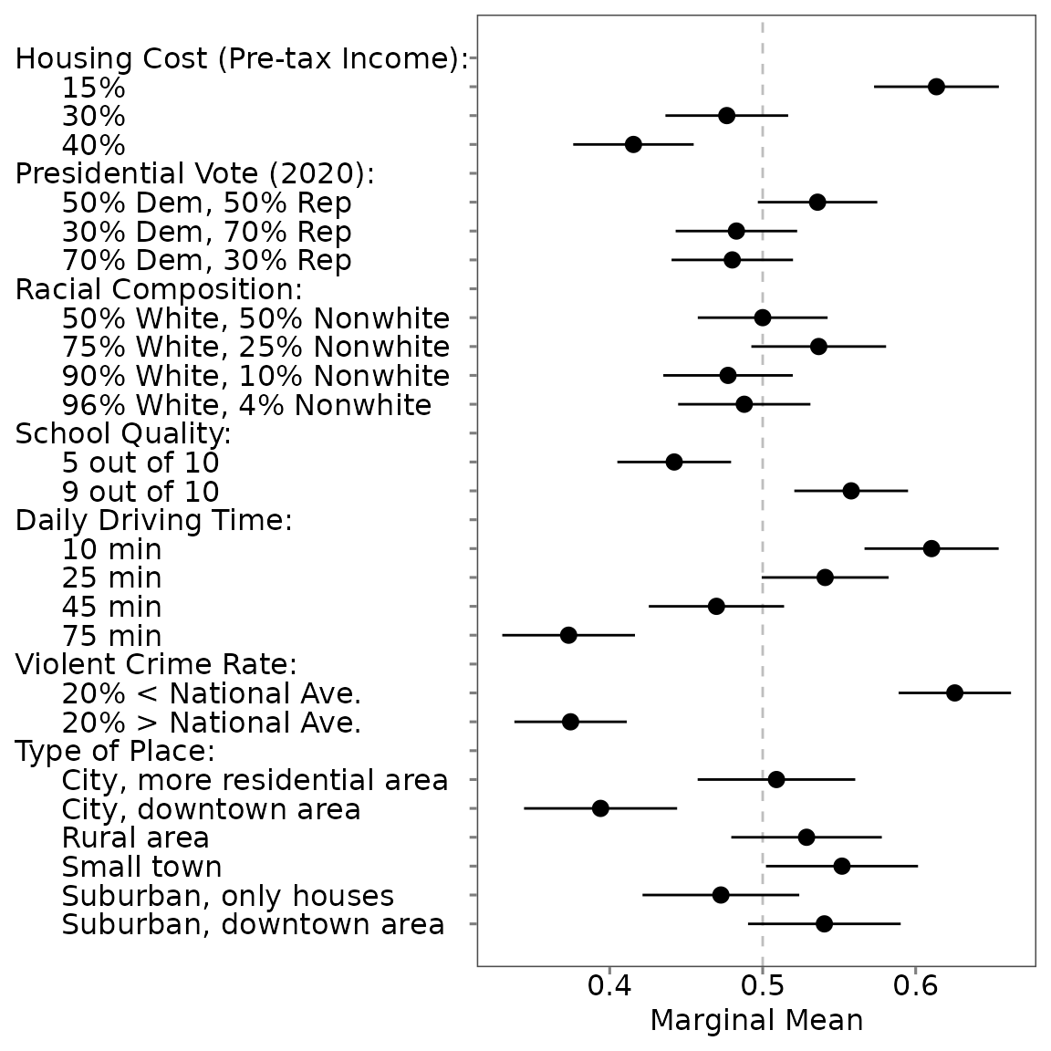
Profile-Level Subgroup Comparison: White vs. Non-White Respondents
outcomes <- c(paste0("choice", 1:8), "choice1_repeated_flipped")

df <- exampleData1 |> mutate(white = ifelse(race == "White", 1, 0))

df_0 <- df |> filter(white == 0) |> reshape_projoint(outcomes)
df_1 <- df |> filter(white == 1) |> reshape_projoint(outcomes)
df_d <- df |> reshape_projoint(outcomes, .covariates = "white")

data_file <- system.file("extdata", "labels_arranged.csv", package = "projoint")
if (data_file == "") stop("File not found!")

df_0 <- read_labels(df_0, data_file)
df_1 <- read_labels(df_1, data_file)
df_d <- read_labels(df_d, data_file)

out_0 <- projoint(df_0, .structure = "profile_level")
out_1 <- projoint(df_1, .structure = "profile_level")
out_d <- projoint(df_d, .structure = "profile_level", .by_var = "white")

plot_0 <- plot(out_0)
plot_1 <- plot(out_1)
plot_d <- plot(out_d, .by_var = TRUE)

plot_0 +
  coord_cartesian(xlim = c(0.2, 0.8)) +
  labs(title = "Non-white", x = "AMCE") +
  theme(plot.title = element_text(hjust = 0.5)) +

plot_1 +
  coord_cartesian(xlim = c(0.2, 0.8)) +
  labs(title = "White", x = "AMCE") +
  theme(axis.text.y = element_blank(), plot.title = element_text(hjust = 0.5)) +

plot_d +
  coord_cartesian(xlim = c(-0.4, 0.4)) +
  labs(title = "Difference", x = "Difference") +
  theme(axis.text.y = element_blank(), plot.title = element_text(hjust = 0.5))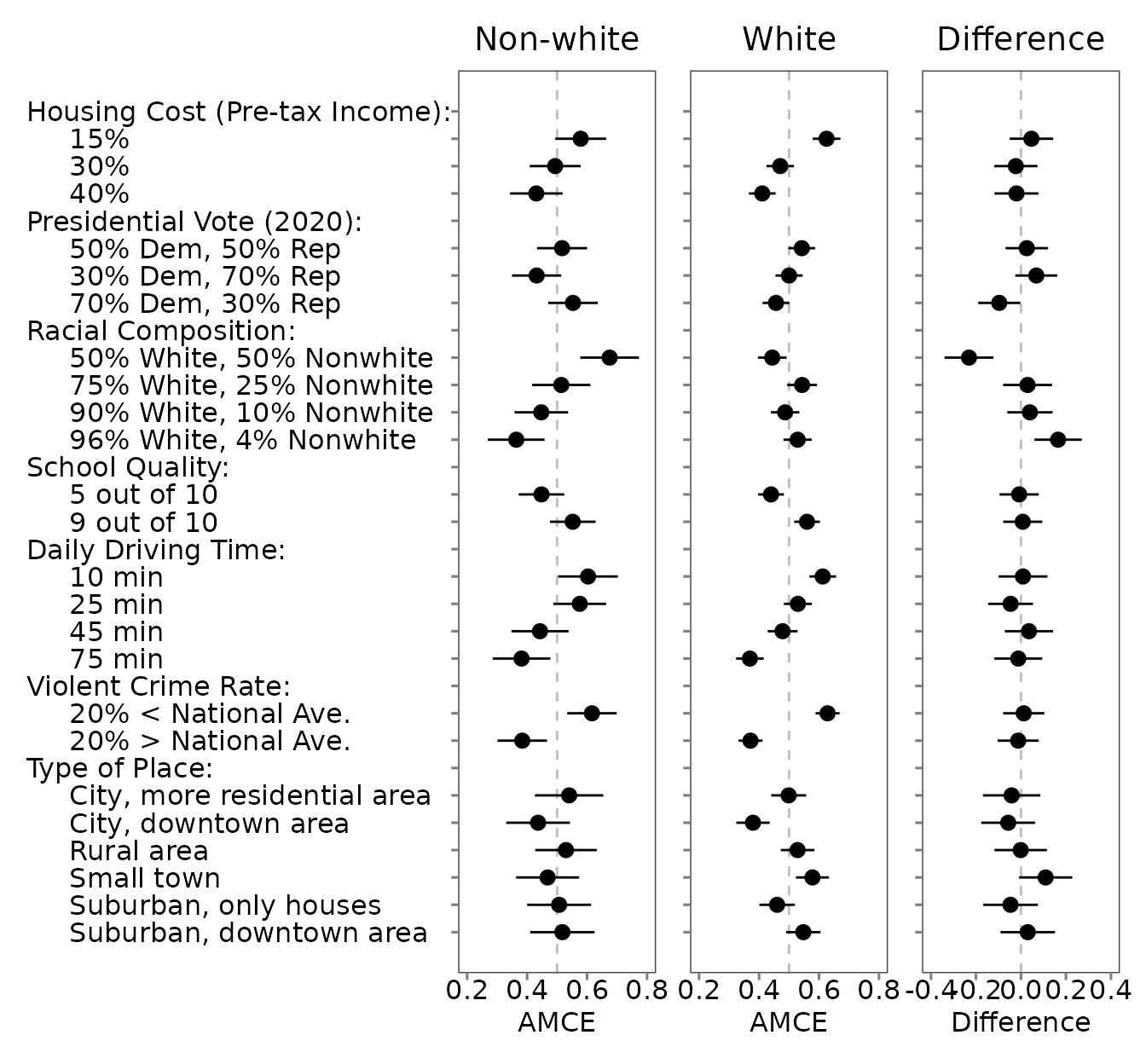
Is there other conjoint software??
See Anton Strezhnev’s Conjoint Survey Design Tool (Link: conjointSDT)
1. Generate a JavaScript or PHP randomizer
Anton Strezhnev’s Conjoint Survey Design Tool (Link: conjointSDT) produces a JavaScript or PHP randomizer.
JavaScript
The JavaScript randomizer can be inserted into the first screen of your Qualtrics survey using Edit Question JavaScript. Example screenshot:

- Example JavaScript: Download here
The JavaScript runs internally within Qualtrics and generates
embedded fields for each conjoint task.
For example:
-
"K-1-1-7"= value for the 7th attribute, first profile, first task -
"K-5-2-5"= value for the 5th attribute, second profile, fifth task
PHP
Alternatively, the PHP randomizer must be hosted externally.
Example hosted on our server:
https://www.horiuchi.org/php/ACHR_Modified_2.php
(PHP file here)
This method was used in:
Agadjanian,
Carey, Horiuchi, and Ryan (2023)
2. Modify your JavaScript or PHP randomizer
You may want to add constraints — for example, prevent
ties between profiles.
To do this, you can manually modify your JavaScript or PHP.
In the future, projoint will offer easier ways to
add constraints!
Until then, resources like OpenAI’s
GPT-4 can help you edit scripts.
Example PHP snippet ensuring racial balance between profiles:
$treat_profile_one = "B-" . (string)$p . "-1-" . (string)$treat_number;
$treat_profile_two = "B-" . (string)$p . "-2-" . (string)$treat_number;
$cond1 = $returnarray[$treat_profile_one] == "White" && $returnarray[$treat_profile_two] == $type;
$cond2 = $returnarray[$treat_profile_two] == "White" && $returnarray[$treat_profile_one] == $type;

if ($cond1 or $cond2) {
  $complete = True;
}
If you have good examples of manual constraints, please email Yusaku Horiuchi!
3. Add conjoint tables with embedded fields in Qualtrics
After generating the randomizer, you must create HTML tables displaying embedded fields for each task.
Example of the first task:

- Example HTML file: task_first.html
Each conjoint study typically includes 5-10 tasks.
The embedded fields update across tasks:
e.g., "K-1..." for Task 1, "K-2..." for Task
2, and so on.
Adding a repeated task (recommended!)
It’s easy to create a repeated task for intra-respondent reliability (IRR) estimation:
- Copy the HTML for Task 1 later into the survey (e.g., after Task 5)
- Flip Profile 1 and Profile 2 (swap the embedded field digits)
Example repeated task:

- Example HTML: task_repeated.html