Wrangle Your Data

🛠️ Wrangle Your Data

Preparing your data correctly is one of the most important steps in conjoint analysis. Fortunately, the reshape_projoint() function in projoint makes this easy.

---

🚀 Quick Workflow

1. Reshape Your Data

Example (Flipped Repeated Task)

outcomes <- paste0("choice", 1:8)
outcomes1 <- c(outcomes, "choice1_repeated_flipped")

out1 <- reshape_projoint(
  .dataframe = exampleData1,
  .outcomes = outcomes1,
  .choice_labels = c("A", "B"),
  .alphabet = "K",
  .idvar = "ResponseId",
  .repeated = TRUE,
  .flipped = TRUE
)

Key Arguments:

• .outcomes: Outcome columns (include repeated task last)
• .choice_labels: Profile labels (e.g., “A”, “B”)
• .idvar: Respondent ID variable
• .alphabet: Variable prefix (“K”)
• .repeated, .flipped: If repeated task exists and is flipped

2. Variations: Repeated vs. Non-Repeated

Not-Flipped Repeated Task

outcomes <- paste0("choice", 1:8)
outcomes2 <- c(outcomes, "choice1_repeated_notflipped")
out2 <- reshape_projoint(
  .dataframe = exampleData2,
  .outcomes = outcomes2,
  .repeated = TRUE,
  .flipped = FALSE
)

No Repeated Task

outcomes <- paste0("choice", 1:8)
out3 <- reshape_projoint(
  .dataframe = exampleData3,
  .outcomes = outcomes,
  .repeated = FALSE
)

3. The .fill Argument: Should You Use It?

Use .fill = TRUE to “fill” missing values based on IRR agreement.

fill_FALSE <- reshape_projoint(
  .dataframe = exampleData1,
  .outcomes = outcomes1,
  .fill = FALSE
)

fill_TRUE <- reshape_projoint(
  .dataframe = exampleData1,
  .outcomes = outcomes1,
  .fill = TRUE
)

Compare:

selected_vars <- c("id", "task", "profile", "selected", "selected_repeated", "agree")
fill_FALSE$data[selected_vars]

## # A tibble: 6,400 × 6
##    id                 task profile selected selected_repeated agree
##    <chr>             <dbl>   <dbl>    <dbl>             <dbl> <dbl>
##  1 R_00zYHdY1te1Qlrz     1       1        1                 1     1
##  2 R_00zYHdY1te1Qlrz     1       2        0                 0     1
##  3 R_00zYHdY1te1Qlrz     2       1        1                NA    NA
##  4 R_00zYHdY1te1Qlrz     2       2        0                NA    NA
##  5 R_00zYHdY1te1Qlrz     3       1        1                NA    NA
##  6 R_00zYHdY1te1Qlrz     3       2        0                NA    NA
##  7 R_00zYHdY1te1Qlrz     4       1        0                NA    NA
##  8 R_00zYHdY1te1Qlrz     4       2        1                NA    NA
##  9 R_00zYHdY1te1Qlrz     5       1        1                NA    NA
## 10 R_00zYHdY1te1Qlrz     5       2        0                NA    NA
## # ℹ 6,390 more rows

fill_TRUE$data[selected_vars]

## # A tibble: 6,400 × 6
##    id                 task profile selected selected_repeated agree
##    <chr>             <dbl>   <dbl>    <dbl>             <dbl> <dbl>
##  1 R_00zYHdY1te1Qlrz     1       1        1                 1     1
##  2 R_00zYHdY1te1Qlrz     1       2        0                 0     1
##  3 R_00zYHdY1te1Qlrz     2       1        1                NA     1
##  4 R_00zYHdY1te1Qlrz     2       2        0                NA     1
##  5 R_00zYHdY1te1Qlrz     3       1        1                NA     1
##  6 R_00zYHdY1te1Qlrz     3       2        0                NA     1
##  7 R_00zYHdY1te1Qlrz     4       1        0                NA     1
##  8 R_00zYHdY1te1Qlrz     4       2        1                NA     1
##  9 R_00zYHdY1te1Qlrz     5       1        1                NA     1
## 10 R_00zYHdY1te1Qlrz     5       2        0                NA     1
## # ℹ 6,390 more rows

Tip:
- Use .fill = TRUE for small-sample or subgroup analysis (helps increase power).
- Use .fill = FALSE (default) when in doubt for safer estimates.

4. What If Your Data Is Already Clean?

If you already have a clean dataset, use make_projoint_data():

out4 <- make_projoint_data(
  .dataframe = exampleData1_labelled_tibble,
  .attribute_vars = c(
    "School Quality", "Violent Crime Rate (Vs National Rate)",
    "Racial Composition", "Housing Cost",
    "Presidential Vote (2020)", "Total Daily Driving Time for Commuting and Errands",
    "Type of Place"
  ),
  .id_var = "id",
  .task_var = "task",
  .profile_var = "profile",
  .selected_var = "selected",
  .selected_repeated_var = "selected_repeated",
  .fill = TRUE
)

Preview:

out4

## <projoint_data>
## - data:     6400 rows, 13 columns
## - labels:   24 levels, 4 columns

5. Arranging Attribute and Level Labels

To reorder or relabel attributes:

1. Save labels:

save_labels(out1, "temp/labels_original.csv")

2. Edit the CSV (change order, label columns; leave level_id untouched)

3. Save it as “labels_arranged.csv” or something else.

4. Reload labels:

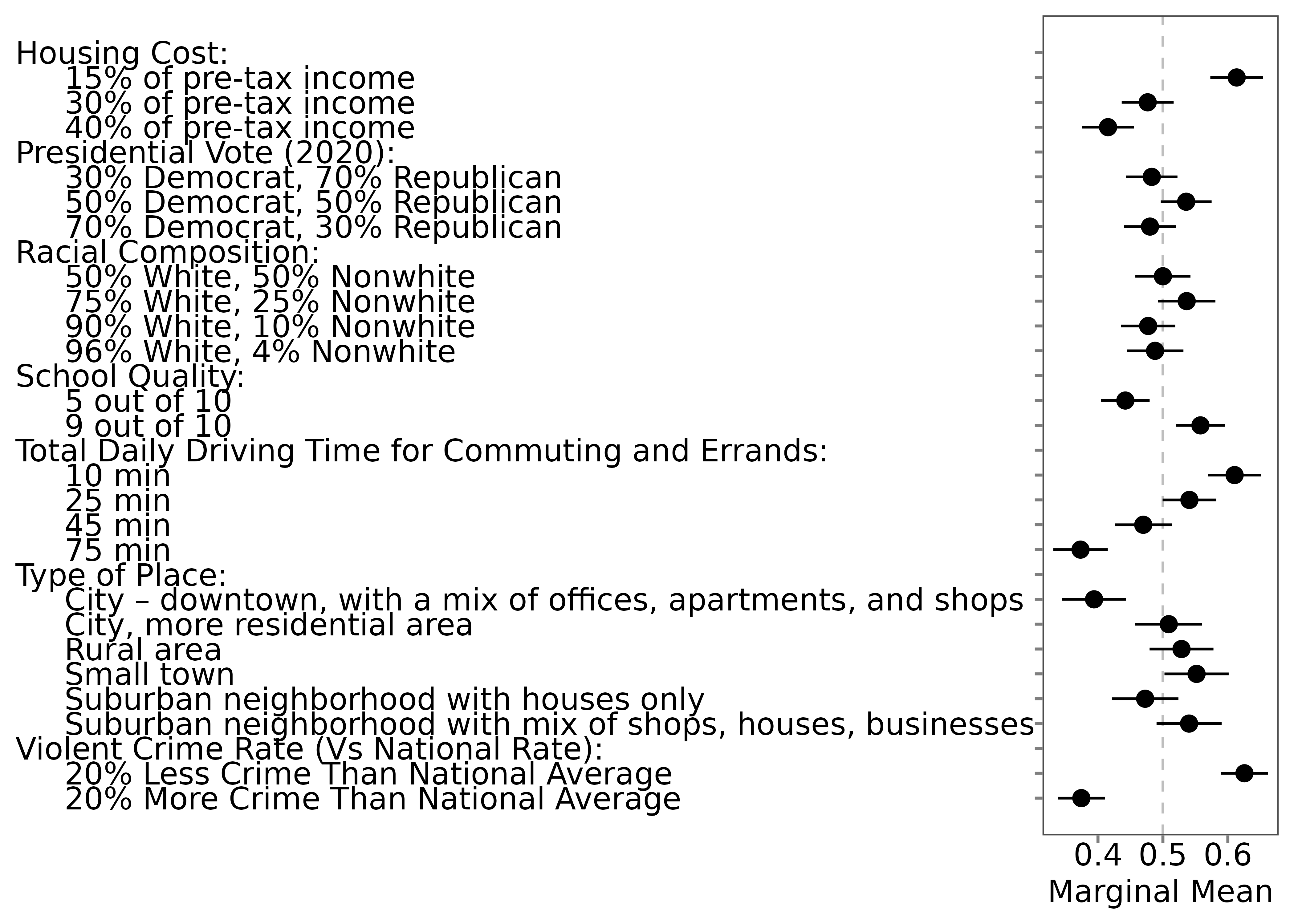
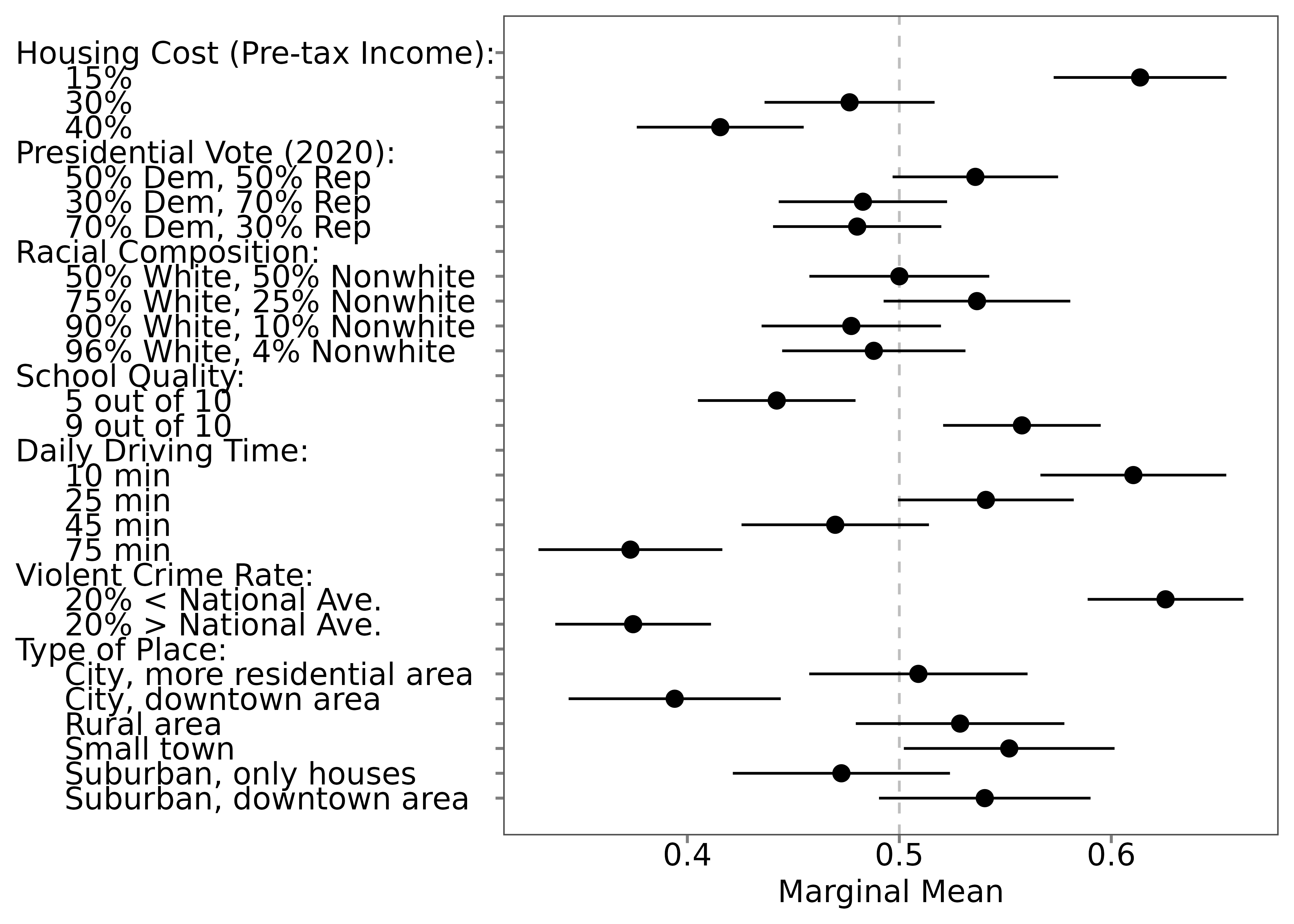
data(out1_arranged, package = "projoint")

Compare using our example:

mm <- projoint(out1, .structure = "profile_level", .estimand = "mm")
plot(mm)

mm <- projoint(out1_arranged, .structure = "profile_level", .estimand = "mm")
plot(mm)

---

🌟 What’s Next?

Now that your data is properly structured, you’re ready to estimate Marginal Means (MMs) or AMCEs!

➡️ Continue to: Analyze Your Conjoint Data
⬅️ Back to: Read Your Qualtrics Data
🏠 Home: Home

---