7. Explore further • projoint

The choice-level analysis will allow researchers to examine many more questions under-investigated in the literature. This article explains some possible avenues for fruitful research.

7.1 Load the projoint package and the other necessary package

library(projoint)
library(ggplot2)

As in the previous articles, we use the already wrangled and cleaned data named “out1_reshaped.” To see what the attribute IDs and level IDs means, you can type:

out1_arranged@labels

## # A tibble: 24 × 4
##    attribute                level                        attribute_id level_id  
##    <chr>                    <chr>                        <chr>        <chr>     
##  1 Housing Cost             15% of pre-tax income        att1         att1:leve…
##  2 Housing Cost             30% of pre-tax income        att1         att1:leve…
##  3 Housing Cost             40% of pre-tax income        att1         att1:leve…
##  4 Presidential Vote (2020) 50% Democrat, 50% Republican att2         att2:leve…
##  5 Presidential Vote (2020) 30% Democrat, 70% Republican att2         att2:leve…
##  6 Presidential Vote (2020) 70% Democrat, 30% Republican att2         att2:leve…
##  7 Racial Composition       50% White, 50% Nonwhite      att3         att3:leve…
##  8 Racial Composition       75% White, 25% Nonwhite      att3         att3:leve…
##  9 Racial Composition       90% White, 10% Nonwhite      att3         att3:leve…
## 10 Racial Composition       96% White, 4% Nonwhite       att3         att3:leve…
## # ℹ 14 more rows

7.1 Examine trade-offs

You may be interested in how people make a choice when they face trade-off options. For example, on the one hand, they may want to live in an inexpensive house. On the other hand, they may prefer to avoid living in an area with a high crime rate. Which of these two options would they prefer? You can compare these two options directly. For the customization of the figure, see Visualize MMs or AMCEs, Choice-level analysis

qoi_1 <- set_qoi(
  .structure = "choice_level",
  .att_choose = "att1", 
  .lev_choose = "level1",
  .att_notchoose = "att6", 
  .lev_notchoose = "level2"
) 

mm1 <- projoint(.data = out1_arranged,
                .qoi = qoi_1,
                .structure = "choice_level", 
                .ignore_position = TRUE)

plot(mm1,
     .labels = c("Housing Cost\n(15% of pre-tax income)", 
                 "Violent Crime Rate\n(20% > National Average)")) +
  labs(y = "Marginal mean",
       x = NULL) +
  coord_cartesian(ylim = c(0, 1)) +
  geom_hline(yintercept = 0.5, 
             linetype = "dashed", 
             color = "darkgray")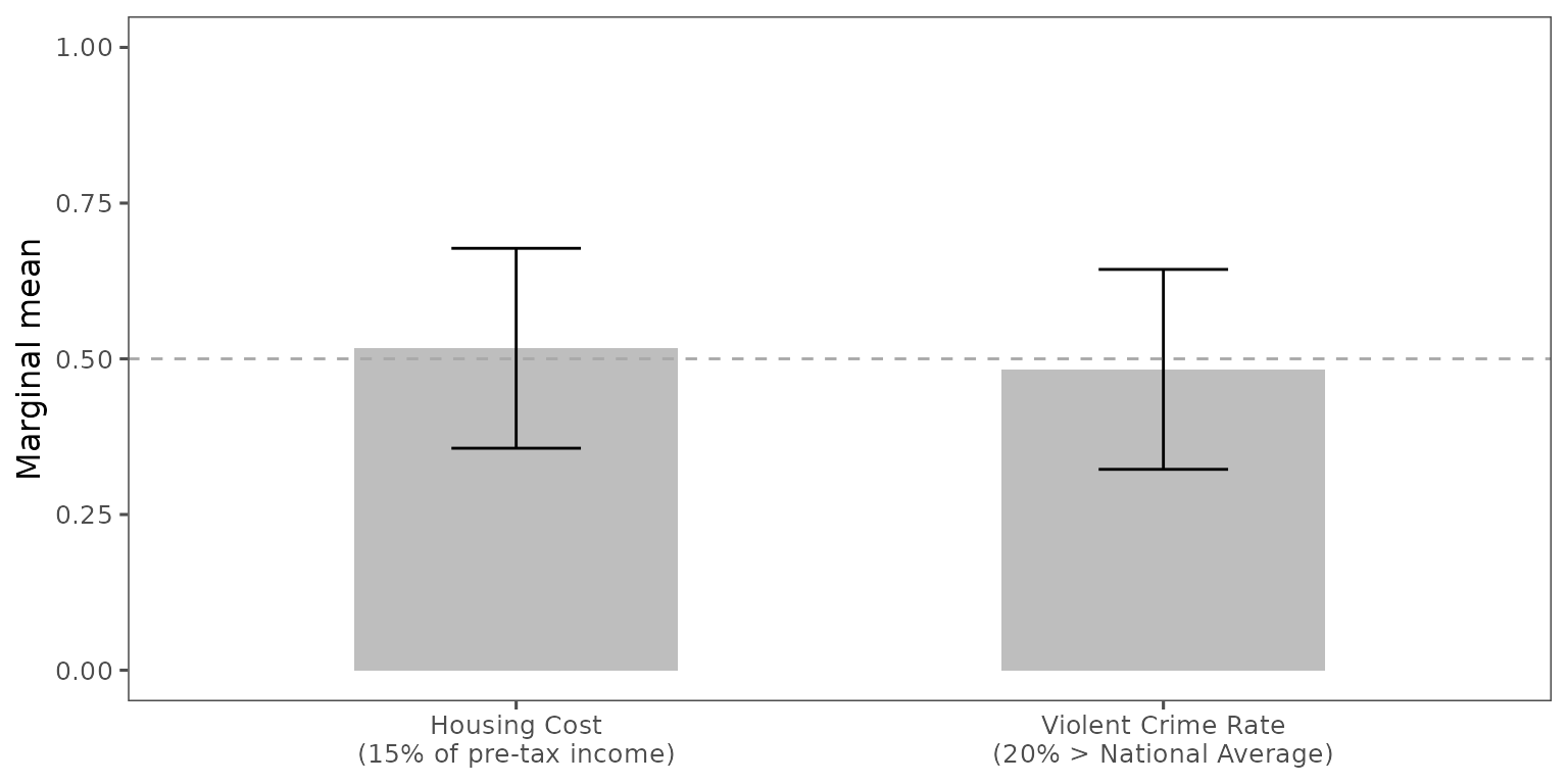

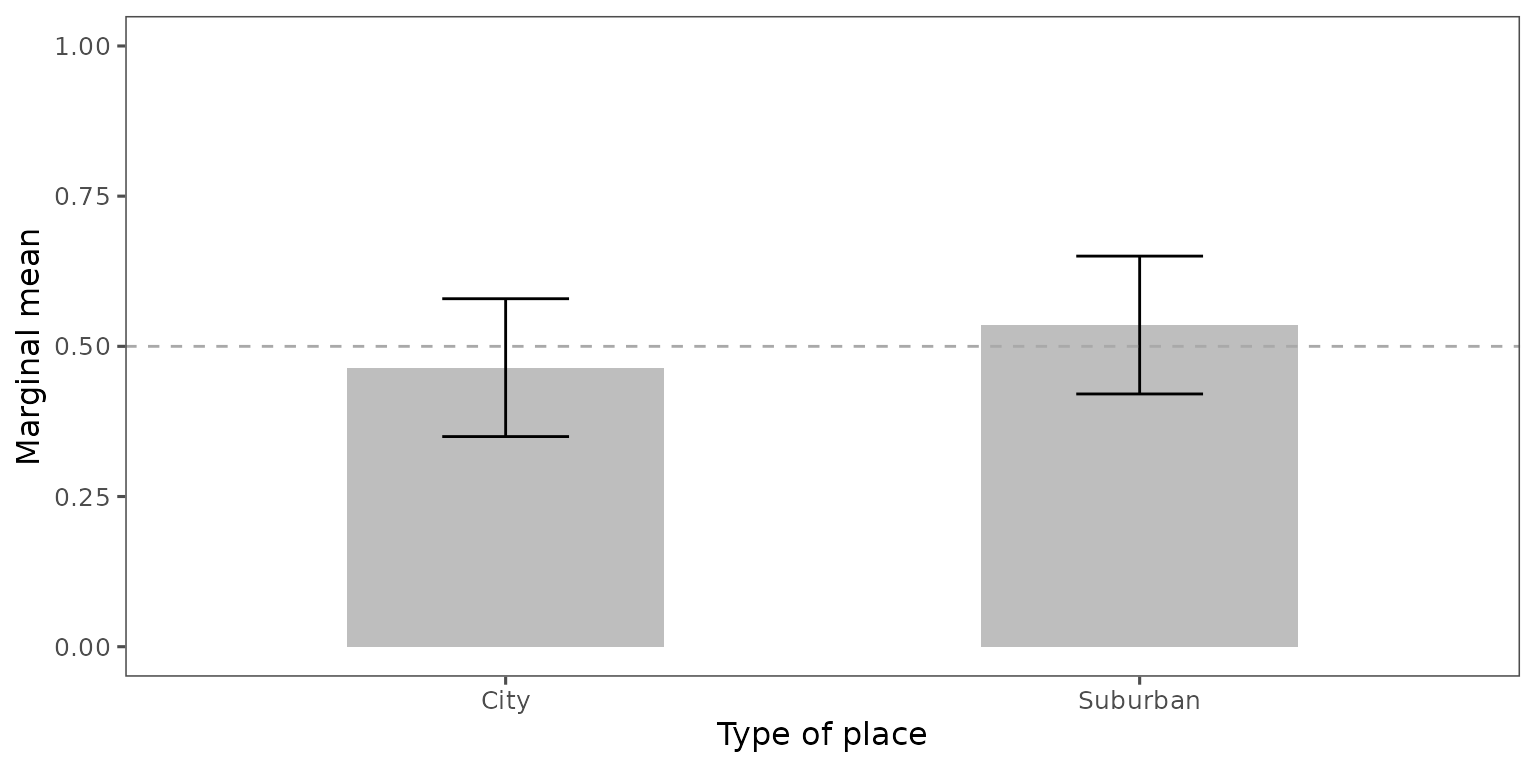
6.1 Set multiple levels for the attribute of interest

You may be interested in measuring the marginal means of choosing more than one level. For example, you may want to estimate the marginal mean of choosing “City, more residential area” OR “City, downtown area” as opposed to “Suburban, only houses” OR “Suburban, downtown area”. Then, you can run the following code:

qoi_2 <- set_qoi(
  .structure = "choice_level",
  .att_choose = "att7", 
  .lev_choose = c("level2", "level3"),
  .att_notchoose = "att7", 
  .lev_notchoose = c("level5", "level6")
)

mm2 <- projoint(.data = out1_arranged,
                .qoi = qoi_2,
                .structure = "choice_level", 
                .ignore_position = TRUE)

plot(mm2, 
     .labels = c("City", "Suburban")) +
  labs(y = "Marginal mean",
       x = "Type of place") +
  coord_cartesian(ylim = c(0, 1)) +
  geom_hline(yintercept = 0.5, 
             linetype = "dashed", 
             color = "darkgray")