3. Predict the intra-respondent reliability (IRR) • projoint

We use two methods to estimate intra-respondent reliability (IRR). The first-best method requires researchers to add a repeated task to their conjoint survey, but is the most reliable. The second method, which uses linear extrapolation, does not require a repeated task but is noisier. If no repeated task is specified, we can use the predict_tau function to perform the extrapolation method and estimate IRR.

3.1 Load the projoint package

library(projoint)

3.2 Predict IRR based on the extrapolation method

As before, start by reading your Qualtrics file and reshaping it using reshape_projoint(). See 2.2 Read and wrangle data, with the flipped repeated tasks. Since we already did that, we’ll skip right ahead and load in the “out1_arranged” object from before. (See 2.5 Arrange the order and labels of attributes and levels.

data(out1_arranged)

We pass this data set to the predict_tau function, which both calculates IRR and produces a figure showing the extrapolation method visually (see 2.3 Arrange the order and labels of attributes and levels).

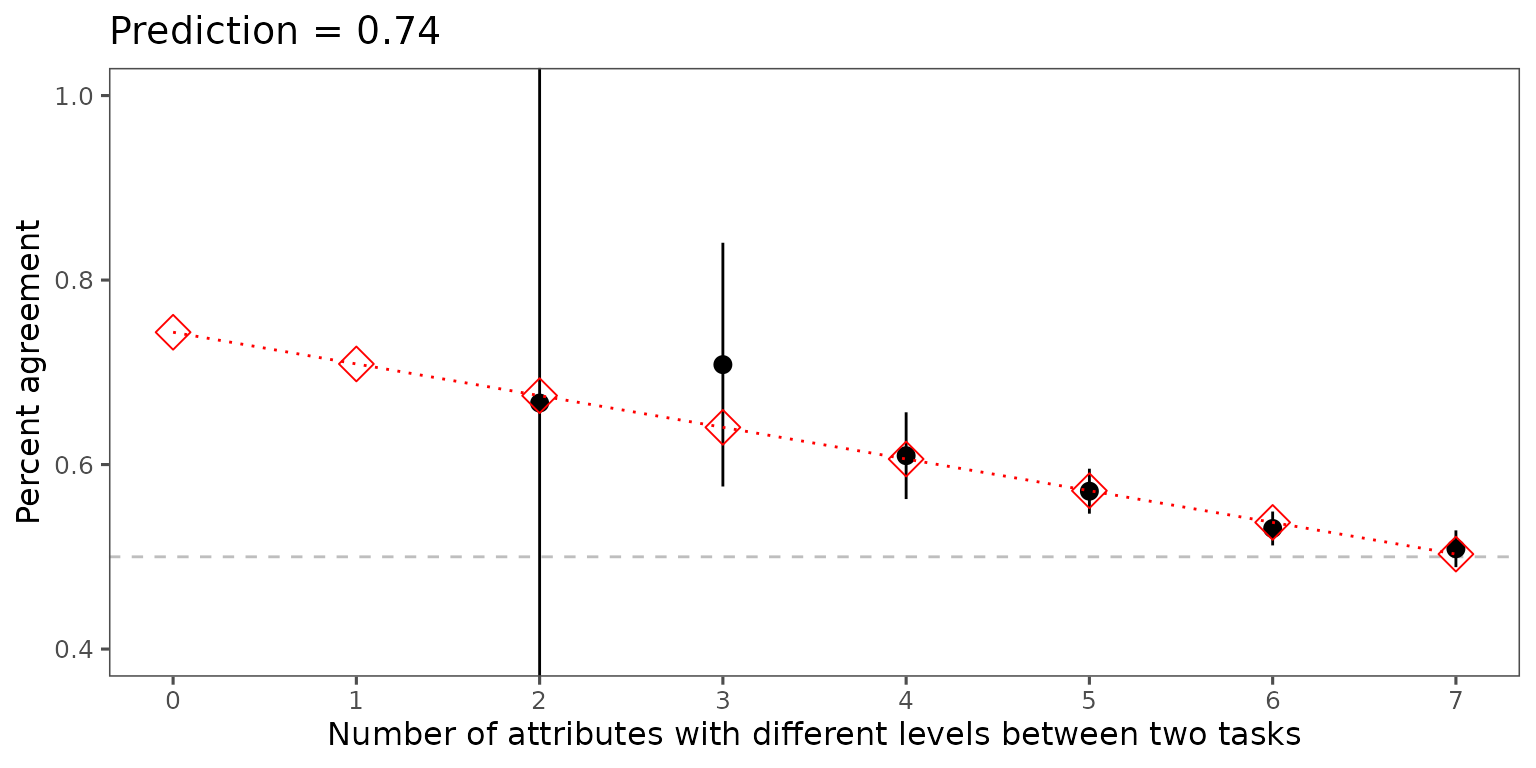
predicted_irr <- predict_tau(out1_arranged)

This projoint_tau object, created by predict_tau, can be explored using the usual tools. The print method explains that this estimate of tau was produced via extrapolation rather than assumed or calculated using a repeated task and presents that estimate:

print(predicted_irr)

## [1] "Tau estimated using the extrapolation method: 0.743"

The summary method returns a tibble of IRR as the profiles become more dissimilar. When x=7, in this example, all attributes are different between the two profiles and we see that IRR is 0.503. We extrapolate to x=0, which is the IRR when both profiles are identical:

summary(predicted_irr)

## # A tibble: 8 × 2
##       x predicted
##   <int>     <dbl>
## 1     0     0.743
## 2     1     0.709
## 3     2     0.675
## 4     3     0.640
## 5     4     0.606
## 6     5     0.572
## 7     6     0.537
## 8     7     0.503

And the plot method renders a plot showing the extrapolated value of tau:

plot(predicted_irr)