2. Read and wrangle your data for conjoint analysis
02-wrangle.RmdMost of the work in analyzing a conjoint task is correctly specifying
the data and columns. In projoint, the
reshape_projoint function makes it easy!
2.2 Read and wrangle data
With the flipped repeated tasks
Let’s look at a simple example. We expand all those arguments below for clarity:
outcomes <- paste0("choice", seq(from = 1, to = 8, by = 1))
outcomes1 <- c(outcomes, "choice1_repeated_flipped")
out1 <- reshape_projoint(.dataframe = exampleData1,
                         .outcomes = outcomes1,
                         .outcomes_ids = c("A", "B"),
                         .alphabet = "K",
                         .idvar = "ResponseId",
                         .repeated = TRUE,
                         .flipped = TRUE,
                         .covariates = NULL,
                         .fill = FALSE)
Let’s walk through the arguments we have specified.
.dataframe is a data frame, ideally read in from Qualtrics
using read_Qualtrics() but not necessarily. The
.idvar argument, a character, indicates that in
exampleData1, the column ResponseId indicates
unique survey respondents. The .outcomes variable lists all
the columns that are outcomes; the last element in this vector is the
repeated task (if it was conducted). .outcomes_ids
indicates the possible options for an outcome; specifically, it is a
vector of characters with two elements, which are the last characters of
the names of the first and second profiles. For example, it should be
c(“A”, “B”) if the profile names are “Candidate A” and “Candidate B”.
This character vector can be anything, such as c(“1”, “2”), c(“a”, “b”),
etc. If you have multiple tasks in your design, you should use the
same profile names across all these tasks. .alphabet
defaults to “K” if the conjoint survey was conducted using either our
tool or Strezhnev’s Conjoint Survey Design
Tool. The final two arguments, .repeated and
.flipped, again relate to the repeated task. If the
.repeated is set to TRUE, then the last
element of the .outcomes vector is taken to be a repetition
of the first task; .flipped indicates whether the profiles
are in the reversed order. See Section 2.3 for .fill.
With the not-flipped repeated tasks
As a slight variation, in some cases the repeated task is
not flipped – that is, in the repeated task, the original
Profile 1 is still Profile 1, rather than flipping positions to Profile
2. Here we specify that by changing .flipped to
FALSE. In the following, we drop the default arguments.
outcomes2 <- c(outcomes, "choice1_repeated_notflipped")
out2 <- reshape_projoint(.dataframe = exampleData2,
                         .outcomes = outcomes2,
                         .repeated = TRUE,
                         .flipped = FALSE)
Without the repeated tasks
Or in cases with no repeated task at all, we set
.repeated to FALSE and .flipped
to NULL. Don’t worry, we can still correct for measurement
error using an extrapolation method; see our third vignette for
details.
out3 <- reshape_projoint(.dataframe = exampleData3,
                         .outcomes = outcomes,
                         .repeated = FALSE)
2.3 The .fill argument
The .fill argument is logical: TRUE if you want to use
information about whether a respondent chose the same profile for the
repeated task and “fill” (using the ‘tidyr’ package) missing values for
the non-repeated tasks, FALSE (otherwise).
You can see the difference by comparing the results of
reshape_projoint when .fill is either
TRUE or FALSE.
fill_FALSE <- reshape_projoint(.dataframe = exampleData1,
                               .outcomes = outcomes1,
                               .fill = FALSE)
fill_TRUE <- reshape_projoint(.dataframe = exampleData1,
                              .outcomes = outcomes1,
                              .fill = TRUE)
Looking only at a subset of the variables, we can see that the first
data frame includes the values for the agree variable
(whether the same profile was chosen or not) only for the repeated task.
The second data frame fills the missing values for the other
non-repeated tasks.
selected_vars <- c("id", "task", "profile", "selected", "selected_repeated", "agree")
fill_FALSE@data[selected_vars]
## # A tibble: 6,400 × 6
## id task profile selected selected_repeated agree
## <chr> <dbl> <dbl> <dbl> <dbl> <dbl>
## 1 R_00zYHdY1te1Qlrz 1 1 1 1 1
## 2 R_00zYHdY1te1Qlrz 1 2 0 0 1
## 3 R_00zYHdY1te1Qlrz 2 1 1 NA NA
## 4 R_00zYHdY1te1Qlrz 2 2 0 NA NA
## 5 R_00zYHdY1te1Qlrz 3 1 1 NA NA
## 6 R_00zYHdY1te1Qlrz 3 2 0 NA NA
## 7 R_00zYHdY1te1Qlrz 4 1 0 NA NA
## 8 R_00zYHdY1te1Qlrz 4 2 1 NA NA
## 9 R_00zYHdY1te1Qlrz 5 1 1 NA NA
## 10 R_00zYHdY1te1Qlrz 5 2 0 NA NA
## # ℹ 6,390 more rows
fill_TRUE@data[selected_vars]## # A tibble: 6,400 × 6
## id task profile selected selected_repeated agree
## <chr> <dbl> <dbl> <dbl> <dbl> <dbl>
## 1 R_00zYHdY1te1Qlrz 1 1 1 1 1
## 2 R_00zYHdY1te1Qlrz 1 2 0 0 1
## 3 R_00zYHdY1te1Qlrz 2 1 1 NA 1
## 4 R_00zYHdY1te1Qlrz 2 2 0 NA 1
## 5 R_00zYHdY1te1Qlrz 3 1 1 NA 1
## 6 R_00zYHdY1te1Qlrz 3 2 0 NA 1
## 7 R_00zYHdY1te1Qlrz 4 1 0 NA 1
## 8 R_00zYHdY1te1Qlrz 4 2 1 NA 1
## 9 R_00zYHdY1te1Qlrz 5 1 1 NA 1
## 10 R_00zYHdY1te1Qlrz 5 2 0 NA 1
## # ℹ 6,390 more rowsIf the number of respondents is small, if the number of specific
profile pairs of your interest is small, and/or if the number of
specific respondent subgroups you want to study is small, it is worth
changing this option to TRUE. But please note that
.fill = TRUE is based on an assumption that IRR is
independent of information contained in conjoint tables. Although our
empirical tests suggest the validity of this assumption, if you are
unsure about it, it is better to use the default value (FALSE).
2.4 What if your data is already clean?
If you have already downloaded your data set from Qualtrics, loaded
it into R, and cleaned it, then you can use
make_projoint_data() to save your data frame or tibble as a
projoint_data object for use with the
projoint(). Here is an example. First, load your data
frame.
data <- exampleData1_labelled_tibbleIt should look like the tibble below. Each row should correspond to
one profile from one task for one respondent. The data frame should have
columns indicating (1) the respondent ID, (2) task number, (3) profile
number, (4) attributes, and (5) a column recording each response (0, 1)
for each task. If your design includes the repeated task, it should also
include a column recording the response for the repeated task. In this
case, that column is select_repeated.
options(tibble.width = Inf)
data
## # A tibble: 6,400 × 14
## id task profile selected selected_repeated `School Quality`
## <chr> <dbl> <dbl> <dbl> <dbl> <chr>
## 1 R_00zYHdY1te1Qlrz 1 1 1 1 9 out of 10
## 2 R_00zYHdY1te1Qlrz 1 2 0 0 5 out of 10
## 3 R_00zYHdY1te1Qlrz 2 1 1 NA 9 out of 10
## 4 R_00zYHdY1te1Qlrz 2 2 0 NA 9 out of 10
## 5 R_00zYHdY1te1Qlrz 3 1 1 NA 5 out of 10
## 6 R_00zYHdY1te1Qlrz 3 2 0 NA 9 out of 10
## 7 R_00zYHdY1te1Qlrz 4 1 0 NA 5 out of 10
## 8 R_00zYHdY1te1Qlrz 4 2 1 NA 9 out of 10
## 9 R_00zYHdY1te1Qlrz 5 1 1 NA 5 out of 10
## 10 R_00zYHdY1te1Qlrz 5 2 0 NA 5 out of 10
## `Violent Crime Rate (Vs National Rate)` `Racial Composition`
## <chr> <chr>
## 1 20% Less Crime Than National Average 50% White, 50% Nonwhite
## 2 20% More Crime Than National Average 50% White, 50% Nonwhite
## 3 20% More Crime Than National Average 90% White, 10% Nonwhite
## 4 20% More Crime Than National Average 96% White, 4% Nonwhite
## 5 20% More Crime Than National Average 96% White, 4% Nonwhite
## 6 20% More Crime Than National Average 90% White, 10% Nonwhite
## 7 20% Less Crime Than National Average 50% White, 50% Nonwhite
## 8 20% Less Crime Than National Average 50% White, 50% Nonwhite
## 9 20% Less Crime Than National Average 75% White, 25% Nonwhite
## 10 20% Less Crime Than National Average 96% White, 4% Nonwhite
## `Housing Cost` `Presidential Vote (2020)`
## <chr> <chr>
## 1 30% of pre-tax income 50% Democrat, 50% Republican
## 2 30% of pre-tax income 70% Democrat, 30% Republican
## 3 30% of pre-tax income 50% Democrat, 50% Republican
## 4 40% of pre-tax income 30% Democrat, 70% Republican
## 5 40% of pre-tax income 70% Democrat, 30% Republican
## 6 30% of pre-tax income 30% Democrat, 70% Republican
## 7 15% of pre-tax income 70% Democrat, 30% Republican
## 8 15% of pre-tax income 50% Democrat, 50% Republican
## 9 15% of pre-tax income 50% Democrat, 50% Republican
## 10 30% of pre-tax income 50% Democrat, 50% Republican
## `Total Daily Driving Time for Commuting and Errands`
## <chr>
## 1 75 min
## 2 10 min
## 3 75 min
## 4 10 min
## 5 10 min
## 6 45 min
## 7 25 min
## 8 10 min
## 9 75 min
## 10 25 min
## `Type of Place` race
## <chr> <fct>
## 1 Suburban neighborhood with houses only White
## 2 City – downtown, with a mix of offices, apartments, and shops White
## 3 Suburban neighborhood with mix of shops, houses, businesses White
## 4 Suburban neighborhood with mix of shops, houses, businesses White
## 5 Rural area White
## 6 Rural area White
## 7 Suburban neighborhood with houses only White
## 8 Suburban neighborhood with mix of shops, houses, businesses White
## 9 City, more residential area White
## 10 City, more residential area White
## ideology
## <fct>
## 1 Moderate; middle of the road
## 2 Moderate; middle of the road
## 3 Moderate; middle of the road
## 4 Moderate; middle of the road
## 5 Moderate; middle of the road
## 6 Moderate; middle of the road
## 7 Moderate; middle of the road
## 8 Moderate; middle of the road
## 9 Moderate; middle of the road
## 10 Moderate; middle of the road
## # ℹ 6,390 more rowsNext, make a character vector of your attributes.
attributes <- c("School Quality",
                "Violent Crime Rate (Vs National Rate)",
                "Racial Composition",
                "Housing Cost",
                "Presidential Vote (2020)",
                "Total Daily Driving Time for Commuting and Errands",
                "Type of Place")
With your data frame and attributes vector, you can use
make_projoint_data() to produce a
projoint_data object. We can see above that the column
indicating the respondent ID is called id, so we pass that
to the .id_var argument of make_projoint_data.
id is also the default for that argument.
out4 <- make_projoint_data(.dataframe = data,
                           .attribute_vars = attributes,
                           .id_var = "id", # the default name
                           .task_var = "task", # the default name
                           .profile_var = "profile", # the default name
                           .selected_var = "selected", # the default name
                           .selected_repeated_var = "selected_repeated", # the default is NULL
                           .fill = TRUE)
The output from this function should look the same as the output of
fill_FALSE in the previous section.
out4## An object of class "projoint_data"
## Slot "labels":
## # A tibble: 24 × 4
## attribute_id level level_id attribute
## <chr> <chr> <chr> <chr>
## 1 att1 15% of pre-tax income att1:lev1 Housing Cost
## 2 att1 30% of pre-tax income att1:lev2 Housing Cost
## 3 att1 40% of pre-tax income att1:lev3 Housing Cost
## 4 att2 30% Democrat, 70% Republican att2:lev1 Presidential Vote (2020)
## 5 att2 50% Democrat, 50% Republican att2:lev2 Presidential Vote (2020)
## 6 att2 70% Democrat, 30% Republican att2:lev3 Presidential Vote (2020)
## 7 att3 50% White, 50% Nonwhite att3:lev1 Racial Composition
## 8 att3 75% White, 25% Nonwhite att3:lev2 Racial Composition
## 9 att3 90% White, 10% Nonwhite att3:lev3 Racial Composition
## 10 att3 96% White, 4% Nonwhite att3:lev4 Racial Composition
## # ℹ 14 more rows
##
## Slot "data":
## # A tibble: 6,400 × 13
## id task profile selected selected_repeated agree att4
## <chr> <dbl> <dbl> <dbl> <dbl> <dbl> <chr>
## 1 R_00zYHdY1te1Qlrz 1 1 1 1 1 att4:lev2
## 2 R_00zYHdY1te1Qlrz 1 2 0 0 1 att4:lev1
## 3 R_00zYHdY1te1Qlrz 2 1 1 NA 1 att4:lev2
## 4 R_00zYHdY1te1Qlrz 2 2 0 NA 1 att4:lev2
## 5 R_00zYHdY1te1Qlrz 3 1 1 NA 1 att4:lev1
## 6 R_00zYHdY1te1Qlrz 3 2 0 NA 1 att4:lev2
## 7 R_00zYHdY1te1Qlrz 4 1 0 NA 1 att4:lev1
## 8 R_00zYHdY1te1Qlrz 4 2 1 NA 1 att4:lev2
## 9 R_00zYHdY1te1Qlrz 5 1 1 NA 1 att4:lev1
## 10 R_00zYHdY1te1Qlrz 5 2 0 NA 1 att4:lev1
## att7 att3 att1 att2 att5 att6
## <chr> <chr> <chr> <chr> <chr> <chr>
## 1 att7:lev1 att3:lev1 att1:lev2 att2:lev2 att5:lev4 att6:lev5
## 2 att7:lev2 att3:lev1 att1:lev2 att2:lev3 att5:lev1 att6:lev1
## 3 att7:lev2 att3:lev3 att1:lev2 att2:lev2 att5:lev4 att6:lev6
## 4 att7:lev2 att3:lev4 att1:lev3 att2:lev1 att5:lev1 att6:lev6
## 5 att7:lev2 att3:lev4 att1:lev3 att2:lev3 att5:lev1 att6:lev3
## 6 att7:lev2 att3:lev3 att1:lev2 att2:lev1 att5:lev3 att6:lev3
## 7 att7:lev1 att3:lev1 att1:lev1 att2:lev3 att5:lev2 att6:lev5
## 8 att7:lev1 att3:lev1 att1:lev1 att2:lev2 att5:lev1 att6:lev6
## 9 att7:lev1 att3:lev2 att1:lev1 att2:lev2 att5:lev4 att6:lev2
## 10 att7:lev1 att3:lev4 att1:lev2 att2:lev2 att5:lev2 att6:lev2
## # ℹ 6,390 more rows2.5 Arrange the order and labels of attributes and levels
By default, reshaped data will have attributes and levels that are ordered alphabetically. If you would like to reorder or relable those attributes or levels, we make that process easy.
You first save the labels using save_labels(), which
produces a CSV file. In that CSV file saved to your local computer, you
should revise the column named order to specify the order
of attributes and levels you want to display in your figure. You can
also revise the labels for attributes and levels in any way you like.
But you should not make any change to the first column named
level_id. After saving the updated CSV file, you can
use read_labels() to read in the modified CSV. We will use
this object later in the projoint function.
save_labels(out1, "temp/labels_original.csv")
out1_arranged <- read_labels(out1, "temp/labels_arranged.csv")
You can find this data set on GitHub: labels_original.csv and labels_arranged.csv.
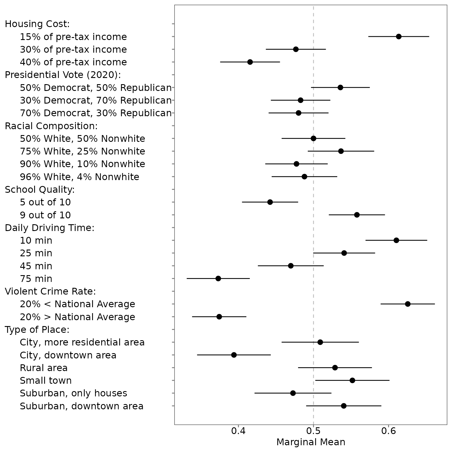
The figure based on the original order and labels is in the alphabetical order:
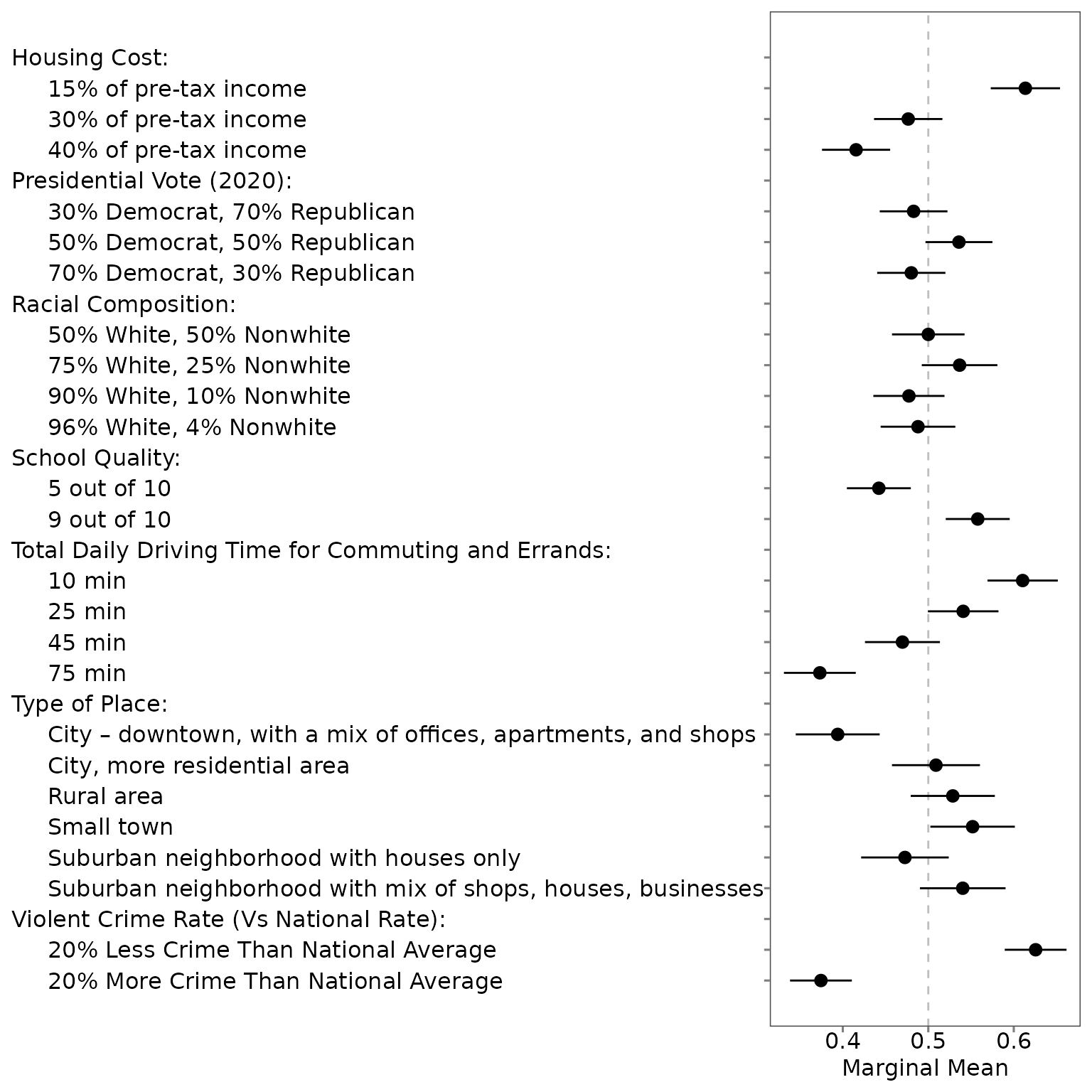
The labels and order of all attribute-levels in the second figure is the same as Figure 2 in Mummolo and Nall (2017).